
Gravity Line Layout
Introduction
The Team’s hard work paid off and we won the contract on a large gravity station survey. Now we actually have to pull it off. I’m the “computer guy” on the team and what they usually need early on is a dataset of GPS points covering the area of interest, and an estimate of the number of stations, which translates into number of survey days, and cost to the Client.
Of course the necessary land access permits have been obtained and now we can design the station layout. The coverage will be a combination of easy access roads, small target grids of high interest, and regional grid points to the edges of the permit area. This post will describe a method of station layout along roads. Grids will come later.
Acquiring Control Points along the Roads
The zeroth step in the process is to translate the Client’s areas of interest into objects on the base map. Using Surfer, I load the base map drawing I described in the previous post Mapping without GIS, and outline these areas in the neighbourhood of Vulcan. Then I’ll apply a reasonable station spacing to the lines and grids. I’ll note that on the drawing. An important detail not to miss: the Client wanted the grid orientation to be NE-SW so that the lines are parallel to the sides of the area. In geology parlance, this is the strike. I’ll choose a line spacing of 100m and a station spacing of 50m so the lines are crossing perpendicular to the direction of strike.

The first step in generating a list of road stations is to digitize a set of control points from the planned layout map. Fortunately, the lines and polygon area added to the base map earlier can be exported to a .bln file containing the control points.
I rounded the coordinates of the vertices to the nearest 10m. For planning purposes, rounding will not affect the accuracy of data at this stage. Final station coordinates will be generated using actual GPS points collected by driving down the road and stopping every few kilometers and at bends.
Note that the first and last point of the grid area are identical. This identifies the object as a closed polygon. We won’t be working with the detailed grid area in this post, just the roads.
12,0
334900,5586800
337080,5588840
337770,5588100
338490,5588780
339850,5587310
339800,5585900  <===> The Detail Grid Area
340490,5585180
339760,5584500
338290,5583140
336890,5583200
335520,5584670
334900,5586800
3,0
333280,5585240
333390,5588480  <===> Road
333440,5589970
3,0
334830,5582050
334930,5585180  <===> Road
335060,5589970
...
Gravline Utility
I wrote a program in C++ called Gravline (download gravline.cpp and download utm.hpp) to generate equally spaced station points following a polyline of control points. I will create an input file for each road in the above .bln file, starting with the first one above. I’ll call it line100.txt, then I’ll run the program in it to create line100.out:
nad27 12  // nad83 or nad27, UTM Zone number
100 0 13  // line, starting station, numbering interval
250.00    // distance between stations in meters
3 UTM     // number of control points, units = UTM or DDEG or DMS
333280  5585240
333390  5588480
333440  5589970
>./gravline line100.txt line100.out
----------------------------
--- GravLine Version 2.1 ---
--- https://biggianthead.ca ---
----------------------------
 Coordinate System: NAD27
 UTM Zone Number: 12
 Line number: 100
 Starting station: 0
 Station interval: 250
 Number of controls: 3
 Format of Control points: Meters
 Control Points (Lat, Long, X, Y):
	50.39750464, -113.34575458	333280.000, 5585240.000
	50.42664998, -113.34564603	333390.000, 5588480.000
	50.44005303, -113.34560452	333440.000, 5589970.000
End of Control Points
line100.out
0	0   50.397505 -113.345755  333280.000 5585240.000  0.000  0.000
0	1   50.426650 -113.345646  333390.000 5588480.000  0.000  0.000
0	2   50.440053 -113.345605  333440.000 5589970.000  0.000  0.000
100	0   50.397505 -113.345755  333280.000 5585240.000  0.000  0.000
100	250   50.399752 -113.345746  333288.483 5585489.856  0.000  0.000
100	500   50.402000 -113.345738  333296.966 5585739.712  0.000  0.000
100	750   50.404247 -113.345729  333305.448 5585989.568  0.000  0.000
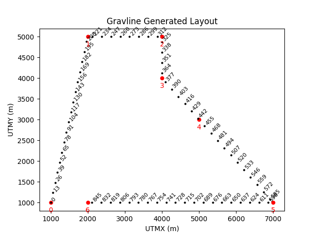
Then I wrote a small Python program using matplotlib.pyplot to plot the line, mostly for debug purposes.

I repeated this process for all the lines. By combining the line*.out files and removing the control points (Line 0), I can post the points onto the planning map in Surfer. In case you think this is a lot of work, you can always write a bash script. It runs in a flash.
|
|
If you have to make changes to any of the digitized lines, just run it again.
This will be a recurring theme: write small utilities that can be chained together, automate as much as you can from start to finish. Make improvements anywhere, then rerun.
Post the Road stations on the project area map
Surfer has a simple method of merging a posted data file that has points in the same coordinate system and that fall within the area of the existing map. You will notice if you look closely, there may be multiple stations within a short distance of each other. The spacing of these regional stations was set to 250m. We don’t want to waste time and money taking readings at duplicate stations like this. What we need to do next is remove the stations that are closer than the minimum distance of 250m. If this sounds like we need to write another program, you would be correct. But we won’t do this right now. We still have to generate a regional grid over the whole visible area of the drawing axes, and another rotated grid within the detail grid, but not to include stations within the centre of town. So we have a lot to do yet. Grids will be the next post. Then we’ll talk about removing unwanted stations after that.
In case you are interested, the allsta.dat file posted on the map has 351 stations, including overlapping coverage for now. The total station count will be a major cost factor to the project, and the Client ultimately pays for the quantity of data collected.

Summary
Gravity survey planning begins with the base map, and translating the Clients needs and wants into a suitable station layout. There are generally 3 sets of data that are collected and merged together to form a gravity dataset:
- detailed grid areas,
- easy to access lines, ie. roads, trails, cut-lines, etc,
- regional stations at a wider spacing, ie. 1 km.
I’ve shown a process of creating a station layout on the base map for easy access lines using small utility programs. Once I’ve generated grid points and removed overlapping stations, they will be added to the layout as well.